Key factors in machine learning research are the speed of the computations and the repeatability of results. Faster computations can boost research efficiency, while repeatability is important for controlling and debugging experiments. For a broad class of machine learning models including neural networks, training computations can be sped up significantly by running on GPUs. However, this speedup is sometimes at the expense of repeatability. For example, in TensorFlow, a popular framework for training machine learning models, repeatability is not guaranteed for a common set of operations on the GPU. Two Sigma researcher Ben Rossi demonstrates this problem for a neural network trained to recognize MNIST digits, and a workaround to enable training the same network on GPUs with repeatable results.
Note that these results were produced on the Amazon cloud with the Deep Learning AMI and TensorFlow 1.0, running on a single NVidia Grid K520 GPU.
Caveat Emptor. The lack of repeatability is often acceptable since the final result (say in terms of out-sample accuracy) is not significantly affected by GPU non-determinism. However, we’ve found that in some applications the final result can be quite different due to this non-determinism. This is because small differences due to GPU non-determinism can accumulate over the course of training, leading to rather different final models. In such cases, the method outlined in this article can be used to ensure repeatability of experiments. However, repeatability achieved with this method is not a panacea since this does not address the fundamental instability of training. A fuller discussion of that is outside the scope of this article, but in our view the chief benefit of repeatability is to ensure that we have accounted for all sources of variation. Once we have that level of control, then we can go back and explore more carefully the stability of training as a function of the source of variation. In particular, even the GPU non-determinism may be explored in this deterministic setting by controlling how mini-batches are constructed. A second benefit of repeatability is that is makes it easier to write regression tests for the training framework.
Non-Determinism with GPU Training
Let us demonstrate the problem on the code to train a simple MNIST network (shown in the Appendix) using the GPU. When we run the code to train the model twice, we obtain the following output.
$ python3 mnist_gpu_non_deterministic.py
epoch = 0 correct = 9557 loss = 0.10369960
epoch = 1 correct = 9729 loss = 0.06410284
epoch = 2 correct = 9793 loss = 0.04644223
epoch = 3 correct = 9807 loss = 0.03983842
epoch = 4 correct = 9832 loss = 0.03518861

$ python3 mnist_gpu_non_deterministic.py
epoch = 0 correct = 9557 loss = 0.10370079
epoch = 1 correct = 9736 loss = 0.06376658
epoch = 2 correct = 9796 loss = 0.04633443
epoch = 3 correct = 9806 loss = 0.03965696
epoch = 4 correct = 9836 loss = 0.03528859
Unfortunately, the output of the second run does not match the output of the first run. In fact, at the end of these two runs, we have two different networks that disagree on at least 4 examples in the test set (9832 correct vs. 9836 correct). Although the difference here is small, as noted above in some applications, there can be a much larger difference.
Narrowing Down the Source of Non-Determinism
Addressing a Known Problem: reduce_sum
We already suspect there is non-determinism in reduce_sum on the GPU from searching Google. Let us verify this is the case, propose an alternative, and verify the alternative does not suffer from the problem. First, note that we have another TensorFlow primitive that does reduction and hopefully does not suffer from non-determinism: matmul. To implement reduce_sum of a column vector as a matrix multiplication, we can multiply its transpose by a column of ones. Below, we show code that applies both reduce_sum and our alternative, reduce_sum_det to a column vector input with 100k elements, 100 times each. We look at the difference between max() and min() of the 100 results for each. For a deterministic computation, we expect this to be zero.
The output for the above script is shown below.
reduce_sum_det mean = 52530.28125000 max-min = 0.000000
reduce_sum mean = 52530.28125000 max-min = 0.019531
The output confirms that reduce_sum is indeed non-deterministic. Encouragingly, we also see that reduce_sum_det always computes the same result. So, let us simply replace reduce_sum with reduce_sum_det. Note that in practice, it is a bit more complicated than this, since we must account correctly for shapes, shown below:
Done, Right? Not Quite.
It turns out that reduce_sum also shows up when computing gradients in our MNIST network, but only for some of the variables. In particular: we see reduce_sum for the bias gradients, but not the weights matrix gradients.
Why does reduce_sum appear when computing bias gradients? If we examine the expression tf.matmul(prev, w) + b in our compute_next function, we see that the matmul term is a matrix whose first dimension is the minibatch size, whereas b is a vector. Therefore, we must broadcast b to the size of the matrix when summing the two terms. Moreover, the gradient for b is back-propagated through this broadcast. When backpropagating gradients through a broadcast, it is necessary to sum the incoming gradients along the axis being broadcast. This is accomplished with reduce_sum, as shown here.
However, there is another way to specify a bias for each network layer that is consistent with how we specify weights, and avoids reduce_sum: we can pack the bias vector into the weights matrix, if we augment the input to each layer with a fixed column of ones. The algebra works out to the same result, with matmul doing the summing for us. Furthermore, matmul has the nice property that its corresponding gradient for either operand is also a matmul, i.e. it is closed under back-propagation.
Putting it Together: Deterministic Training on the GPU
The following is the output of running the deterministic training script twice:
$ python3 mnist_gpu_deterministic.py
epoch = 0 correct = 9582 loss = 0.10278721
epoch = 1 correct = 9734 loss = 0.06415118
epoch = 2 correct = 9798 loss = 0.04612210
epoch = 3 correct = 9818 loss = 0.03934029
epoch = 4 correct = 9840 loss = 0.03456130

$ python3 mnist_gpu_deterministic.py
epoch = 0 correct = 9582 loss = 0.10278721
epoch = 1 correct = 9734 loss = 0.06415118
epoch = 2 correct = 9798 loss = 0.04612210
epoch = 3 correct = 9818 loss = 0.03934029
epoch = 4 correct = 9840 loss = 0.03456130
Success! The two runs perfectly match.
Conclusions and Discussion
We confirmed that reduce_sum is non-deterministic on the GPU, and found a workaround using matmul. However, we could not simply replace reduce_sum with our deterministic version, since reduce_sum shows up in the gradient computation whenever a broadcast is involved. To work around this, we switched to augmenting layer inputs with a column of ones and storing biases in our weights matrix.
How do we know that matmul is truly deterministic and not simply less non-deterministic than reduce_sum? Are there guarantees? In TensorFlow, the matmul operation on the GPU relies on NVidia’s cuBLAS library, and the cuBLAS documentation says that “by design, all CUBLAS API routines from a given toolkit version generate the same bit-wise results at every run when executed on GPUs with the same architecture and the same number of SMs.” So, we can indeed rely on matmul to provide repeatable results.
Note that while this result may be useful to others writing fully connected TensorFlow networks and training them from scratch, it may not apply to higher level frameworks that ultimately rely on the TensorFlow operations that are non-deterministic.
As a final question, why does TensorFlow have non-deterministic behavior by default? Operations like reduce_sum can be faster than matmul since they rely on CUDA atomics. Though this speedup depends on the size of the data and the surrounding computation, presumably there is enough of a speedup in many cases to justify the loss of repeatability, particularly when the application is not sensitive to non-determinism.
Appendix: MNIST Data, Network and Training Code
MNIST Data
We download and gunzip the MNIST image and label data from Yann Lecun’s website.
Load into Numpy Array in Python
With numpy we can mmap the ND array data in as-is.
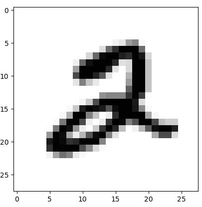
We can verify we’ve loaded the data correctly with matplotlib.
Preprocess Data for Net
Before training a network, we scale the pixel values to the range 0 – 1 and transform the labels into a “one hot” representation.
Network Construction (Non-Deterministic)
We construct a fully-connected neural network to classify MNIST digits with two hidden layers of size 1000 each. We set the input to have a dynamic shape (None). This is useful to be able to run the same network both for training with minibatches and inference on a single example.
We use minibatches of size 1000 and Adam to optimize the loss, which is the mean squared error (MSE) between the target classes and the network outputs.
Network Construction (Deterministic)
To correct for the behavior of reduce_sum and non-deterministic reduction when broadcasting biases, as described in the main article we implement our own version of reduce_sum that uses matmul, and we implement biases by augmenting the weights matrix as well as all previous layer inputs with a ones column.
Training Code (SGD)
Source
The complete source code for the deterministic and non-deterministic MNIST experiments is available under the Apache License, version 2.0: